Let’s assume that we want generate samples from a multivariate normal distribution.

First we assume we know how to generate samples from a univariate gaussian distribution.

So we have n independent random variables $x_1, x_2,…, x_d$ where $x_i \sim \mathcal{N(0,1)}$

$\langle \vec{x} \rangle =0$ and $\langle \vec{x} \vec{x}^T \rangle = \mathbb{1}$.

and what we aim to find is a linear mapping $M: \vec{x} \mapsto \vec{y}$.

Where the new variable $y$ has a covariance matrix $C$, where $C=\langle \vec{y} \vec{y}^T\rangle$ which we can specify as we wish, remember though that a covariance matrix has to be positive definite.

So we want to find a transformation matrix $M$ where $M \vec{x} = \vec{y}$.

$C = \langle \vec{y} \vec{y}^T\rangle = \langle M \vec{x} (M \vec{x})^\intercal\rangle = \langle M \vec{x} \vec{x}^\intercal M^\intercal \rangle = M \langle \vec{x} \vec{x}^\intercal \rangle M^\intercal = M M^\intercal $.

Now let’s remember that the covariance matrix $C$ has to be a symmetric(hermitian) and positive definite matrix. For those kind of matrices we can always decompose it into the product of a lower triangular matrix $L$ and its transpose $L^\intercal$ [https://en.wikipedia.org/wiki/Cholesky_decomposition].

$ C = L \ L^T$

This is called the Cholesky decomposition.

So $L=M$ and we simply have to find the Cholesky decomposition, $L$, of our desired covariance matrix $C$ and apply it to our univariate gaussian samples.

We can easily generate samples from a univariate normal distribution:

import numpy as np 
import matplotlib.pyplot as plt
import seaborn as sns


d = 2
n = 100000 

# first we create our samples from the 2 independent normal distributions
x = np.random.normal(loc=0, scale=1, size=d*n).reshape(d, n)



# now we specify our covariance matrix
K_0 = np.array([[2, 1],
                [1, 2]])
# we calculate the Cholesky deomposition - L is the lower diagonal matrix
L = np.linalg.cholesky(K_0) 
y = np.dot(L, x)

# now let's see how samples from our new distribution looks like
sns.jointplot(x=x[0],
              y=x[1], 
              kind="kde", 
              space=0)


# we can compare our generated samples to the samples we get from the numpy function multivariate_normal
mean = [0, 0]
z = np.random.multivariate_normal(mean,cov=K_0, size=n)
y = np.transpose(z)

sns.jointplot(x=y[0],
              y=y[1], 
              kind="kde", 
              space=0);

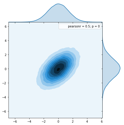
Here we see the distribution from our code using Cholesky decomposition:

Here we see the distribution from the numpy function multivariate_normal

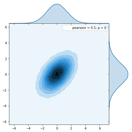
And we see that they are identical so this seems to work

##