Transfer Learning Using A Convolutional Neural Network
Transfer learning is using a neural network which has been trained for solving a specific task and applying to a different problem. For example in this paper from 2017 a neural network was pre-trained on the ImageNet dataset with 1000 classes. That network was then trained to classify images of skin lesions, which are completely different from the 1000 classes in ImageNet.
Of course the network is not completely ready to start solving the new task, we have to perform some optimization and change the structure of the network at least a little bit. But the changes can be bound to the last layer.
I recently wrote a blogpost about applying a neural network to classify images of cats and dogs. There I got accuracy of 0.83 - let’s see if we can get better results for this task by using transfer learning.
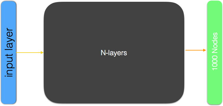
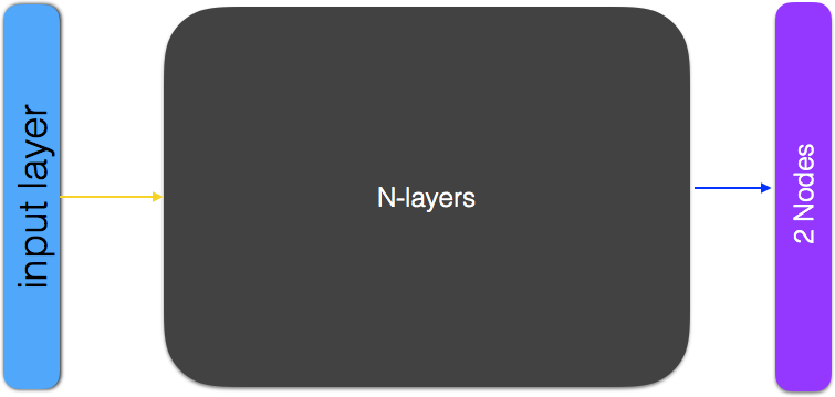
Tensorflow has a collection of pretrained models which we can use to do transfer learning. We will use the MobileNetV2 which has been trained on the ImageNet dataset. However since ImageNet has 1000 classes the output layer in MobileNetV2 has 1000 nodes. We remove the last layer and replace it with an output layer of 2 nodes and we only train the last layer. Tensorflow Hub makes this easy for us since it allows us to download pretrained networks where the last layer has been removed. We can simply append our last layer of choice to the network, set the rest of the network to trainable=False and start training the last layer. This can give remarkably good results.
Here we see an abstraction of the methodology:
Like before we stary by importing the neccessary libraries (for more detailed description of the code, please see my previous blog)
from __future__ import absolute_import, division, print_function, unicode_literals

try:
  # Use the %tensorflow_version magic if in colab.
  %tensorflow_version 2.x
except Exception:
  pass

import tensorflow as tf
from tensorflow.keras.preprocessing.image import ImageDataGenerator
import os
import numpy as np
import matplotlib.pyplot as plt
from tensorflow.keras import layers
TensorFlow 2.x selected.
_URL = 'https://storage.googleapis.com/mledu-datasets/cats_and_dogs_filtered.zip'

zip_dir = tf.keras.utils.get_file('cats_and_dogs_filterted.zip', origin=_URL, extract=True)

base_dir = os.path.join(os.path.dirname(zip_dir), 'cats_and_dogs_filtered')
train_dir = os.path.join(base_dir, 'train')
validation_dir = os.path.join(base_dir, 'validation')
print(zip_dir)
/root/.keras/datasets/cats_and_dogs_filterted.zip
train_cats_dir = os.path.join(train_dir, 'cats')
train_dogs_dir = os.path.join(train_dir, 'dogs')
validation_cats_dir = os.path.join(validation_dir, 'cats')
validation_dogs_dir = os.path.join(validation_dir, 'dogs')
We see that the training set is small (1000 images of each class) as well as the test set.
num_cats_tr = len(os.listdir(train_cats_dir))
num_dogs_tr = len(os.listdir(train_dogs_dir))

num_cats_val = len(os.listdir(validation_cats_dir))
num_dogs_val = len(os.listdir(validation_dogs_dir))

total_train = num_cats_tr + num_dogs_tr
total_val = num_cats_val + num_dogs_val

print('total training cat images:', num_cats_tr)
print('total training dog images:', num_dogs_tr)

print('total validation cat images:', num_cats_val)
print('total validation dog images:', num_dogs_val)
print("--")
print("Total training images:", total_train)
print("Total validation images:", total_val)
total training cat images: 1000
total training dog images: 1000
total validation cat images: 500
total validation dog images: 500
--
Total training images: 2000
Total validation images: 1000
MobileNetV2 takes as input figures of size 224*224 so we have to adjust our images to that size.
import cv2
train_cats_dir = os.path.join(train_dir, 'cats')

im1 = cv2.imread(train_cats_dir+"/cat.0.jpg")
im2 = cv2.imread(train_cats_dir+"/cat.1.jpg")

print(type(im1), type(im2))
print(im1.shape, im2.shape)
IMG_SHAPE = 224
<class 'numpy.ndarray'> <class 'numpy.ndarray'>
(374, 500, 3) (280, 300, 3)
train_image_generator      = ImageDataGenerator(rescale=1./255)
validation_image_generator = ImageDataGenerator(rescale=1./255)
BATCH_SIZE = 100 # number of samples to use to calculate the gradient at each update step.
Like I went through in detail in my previous CNN blog post we augment our training dataset by tweaking(shifting, rotating and more) the images using the class ImageDataGenerator.
image_gen_train = ImageDataGenerator(
      rescale=1./255,
      rotation_range=40,
      width_shift_range=0.2,
      height_shift_range=0.2,
      shear_range=0.2,
      zoom_range=0.2,
      horizontal_flip=True,
      fill_mode='nearest')

train_data_gen = image_gen_train.flow_from_directory(batch_size=BATCH_SIZE,
                                                     directory=train_dir,
                                                     shuffle=True,
                                                     target_size=(IMG_SHAPE,IMG_SHAPE),
                                                     class_mode='binary')
Found 2000 images belonging to 2 classes.
The validation dataset is not tweaked, simply rescaled.
image_gen_val = ImageDataGenerator(rescale=1./255)

val_data_gen = image_gen_val.flow_from_directory(batch_size=BATCH_SIZE,
                                                 directory=validation_dir,
                                                 target_size=(IMG_SHAPE, IMG_SHAPE),
                                                 class_mode='binary')
Found 1000 images belonging to 2 classes.
Now we download the MobileNetV2 convolutional neural network, where the last layer has been removed. Note that if we would have liked to get the last layer included in the model we would have used the link “https://tfhub.dev/google/tf2-preview/mobilenet_v2/classification/2”.
import tensorflow_hub as hub

URL = "https://tfhub.dev/google/tf2-preview/mobilenet_v2/feature_vector/2"
feature_extractor = hub.KerasLayer(URL,
                                   input_shape=(IMG_SHAPE, IMG_SHAPE,3))
We want to keep all the parameters in the models as they are and only optimize the last layer, so we set the parameters in the MobileNet network to non trainable.
feature_extractor.trainable = False
Finally we append a dense layer of 2 nodes to the MobileNet network (feature_extractor).
model = tf.keras.Sequential([
  feature_extractor,
  layers.Dense(2)
])

model.summary()
Model: "sequential"
_________________________________________________________________
Layer (type)                 Output Shape              Param #
=================================================================
keras_layer (KerasLayer)     (None, 1280)              2257984
_________________________________________________________________
dense (Dense)                (None, 2)                 2562
=================================================================
Total params: 2,260,546
Trainable params: 2,562
Non-trainable params: 2,257,984
_________________________________________________________________
Now we can simply start training the model.
model.compile(
  optimizer='adam',
  loss=tf.keras.losses.SparseCategoricalCrossentropy(from_logits=True),
  metrics=['accuracy'])

EPOCHS = 6

history = model.fit_generator(
    train_data_gen,
    steps_per_epoch=int(np.ceil(total_train / float(BATCH_SIZE))),
    epochs=EPOCHS,
    validation_data=val_data_gen,
    validation_steps=int(np.ceil(total_val / float(BATCH_SIZE)))
)
Let’s plot the performance of the model as a function of epochs.
acc = history.history['accuracy']
val_acc = history.history['val_accuracy']

loss = history.history['loss']
val_loss = history.history['val_loss']

epochs_range = range(EPOCHS)

plt.figure(figsize=(8, 8))
plt.subplot(1, 2, 1)
plt.plot(epochs_range, acc, label='Training Accuracy')
plt.plot(epochs_range, val_acc, label='Validation Accuracy')
plt.legend(loc='lower right')
plt.title('Training and Validation Accuracy')

plt.subplot(1, 2, 2)
plt.plot(epochs_range, loss, label='Training Loss')
plt.plot(epochs_range, val_loss, label='Validation Loss')
plt.legend(loc='upper right')
plt.title('Training and Validation Loss')
plt.show()
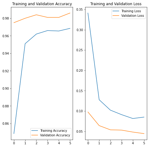
The accuracy of the validation set is around 0.99, in comparison the accuracy of the validation set in the previous blog post was around 0.83 . We also note that the accuracy in the training set is lower than in the validation set, this could be due to the fact that the training set contains augmented images which might be harder to classify then images in the validation set.
All in all see that by using this pretrained model we get much higher accuracy with minimal effort.