Overcoming Overfitting In Convolutional Neural Networks
When using convolutional neural networks (CNNs) it’s easy to run into the problem of overfitting. However there are a few things we can do to tackle this problem and here I intend to demonstrate the effectiveness of a couple of them.
- Explore the Dataset
- Data Preparation
- Defining the network
- Training the model
- Data Augmentation
- Final augmented dataset
- Improving the model - Dropout
- Results of improved model
Our task is to classify images of cats and dogs, using a convolutional neural network. Sounds easy enough. We start by downloading a dataset(or part of it) from Microsoft Research.
from __future__ import absolute_import, division, print_function, unicode_literals

try:
  # Use the %tensorflow_version magic if in colab.
  %tensorflow_version 2.x
except Exception:
  pass

import tensorflow as tf
from tensorflow.keras.preprocessing.image import ImageDataGenerator
import os
import numpy as np
import matplotlib.pyplot as plt
TensorFlow 2.x selected.
_URL = 'https://storage.googleapis.com/mledu-datasets/cats_and_dogs_filtered.zip'

zip_dir = tf.keras.utils.get_file('cats_and_dogs_filterted.zip', origin=_URL, extract=True)

base_dir = os.path.join(os.path.dirname(zip_dir), 'cats_and_dogs_filtered')
train_dir = os.path.join(base_dir, 'train')
validation_dir = os.path.join(base_dir, 'validation')
print(zip_dir)
/root/.keras/datasets/cats_and_dogs_filterted.zip
Now we have extracted all the data needed, now let’s assign each directory to a variable.
train_cats_dir = os.path.join(train_dir, 'cats')
train_dogs_dir = os.path.join(train_dir, 'dogs')
validation_cats_dir = os.path.join(validation_dir, 'cats')
validation_dogs_dir = os.path.join(validation_dir, 'dogs')
Explore the Dataset
Now that we have downloaded the data let’s see how many figures we have
of cats and dogs in the training and validation set.
num_cats_tr = len(os.listdir(train_cats_dir))
num_dogs_tr = len(os.listdir(train_dogs_dir))

num_cats_val = len(os.listdir(validation_cats_dir))
num_dogs_val = len(os.listdir(validation_dogs_dir))

total_train = num_cats_tr + num_dogs_tr
total_val = num_cats_val + num_dogs_val

print('total training cat images:', num_cats_tr)
print('total training dog images:', num_dogs_tr)

print('total validation cat images:', num_cats_val)
print('total validation dog images:', num_dogs_val)
print("--")
print("Total training images:", total_train)
print("Total validation images:", total_val)
total training cat images: 1000
total training dog images: 1000
total validation cat images: 500
total validation dog images: 500
--
Total training images: 2000
Total validation images: 1000
Let’s take a look at the dimensions of a couple of figures:
import cv2
train_cats_dir = os.path.join(train_dir, 'cats')

im1 = cv2.imread(train_cats_dir+"/cat.0.jpg")
im2 = cv2.imread(train_cats_dir+"/cat.1.jpg")

print(type(im1), type(im2))
print(im1.shape, im2.shape)
<class 'numpy.ndarray'> <class 'numpy.ndarray'>
(374, 500, 3) (280, 300, 3)
We see that they don’t have the same size. However we can simply resize the figures later. Let’s define the target size as 150 pixels.
IMG_SHAPE = 150
Data Preparation
Now we would like to read all the images into 3-dimensional tensors (floating point). Then we scale the tensor values from values between 0 and 255 to values between 0 and 1.
We can do just that in a really easy way using the class tf.keras.preprocessing.image.ImageDataGenerator.
train_image_generator      = ImageDataGenerator(rescale=1./255)
validation_image_generator = ImageDataGenerator(rescale=1./255)
the method flow_from_directory will load images from the disk for each batch it will also rescale the pixel values using the rescale factor we defined above, and resize the figures to IMG_SHAPE a using single line of code.
BATCH_SIZE = 100 # number of samples to use to calculate the gradient at each update step.
train_data_gen = train_image_generator.flow_from_directory(batch_size=BATCH_SIZE,
                                                           directory=train_dir,
                                                           shuffle=True,
                                                           target_size=(IMG_SHAPE,IMG_SHAPE),
                                                           class_mode='binary')
Found 2000 images belonging to 2 classes.
val_data_gen = validation_image_generator.flow_from_directory(batch_size=BATCH_SIZE,
                                                              directory=validation_dir,
                                                              shuffle=False,
                                                              target_size=(IMG_SHAPE,IMG_SHAPE), #(150,150)
                                                              class_mode='binary')
Found 1000 images belonging to 2 classes.
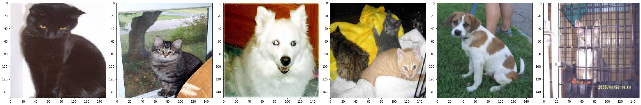
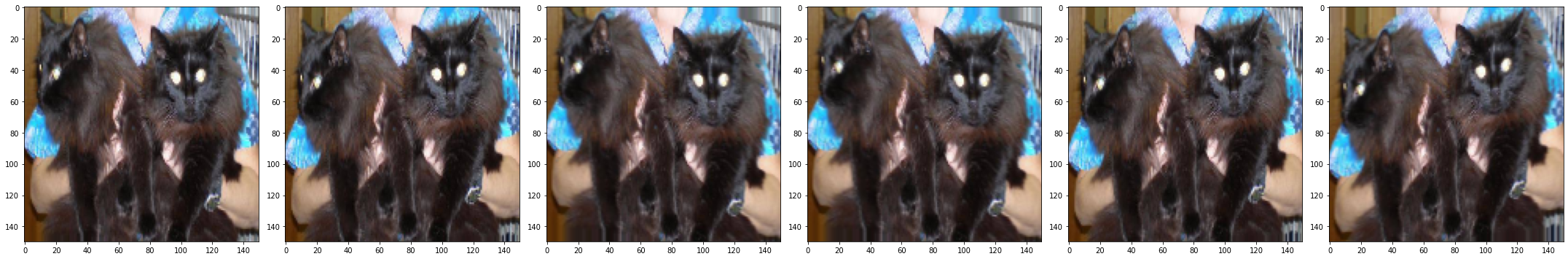
Let’s display a few of the figures. First we get the next batch from the generator train_data_gen.
sample_training_images, _ = next(train_data_gen)
def plotImages(images_arr, n):
    fig, axes = plt.subplots(1, n, figsize=(30,30))
    for img, ax in zip(images_arr, axes):
        ax.imshow(img)
    plt.tight_layout()
    plt.show()
plotImages(sample_training_images[:6], 6)
Defining the network
The network has four layers of convolution blocks, and we apply a max pool layer after each of the convolution blocks. Finally there is a fully connected layer with 512 units and the final ouput has two units (cats and dogs) which we can view as logits. We can then transform these logits to probabilities using the softmax function.
model = tf.keras.models.Sequential([
    tf.keras.layers.Conv2D(32, (3,3), activation='relu', input_shape=(150, 150, 3)),
    tf.keras.layers.MaxPooling2D(2, 2),

    tf.keras.layers.Conv2D(64, (3,3), activation='relu'),
    tf.keras.layers.MaxPooling2D(2,2),

    tf.keras.layers.Conv2D(128, (3,3), activation='relu'),
    tf.keras.layers.MaxPooling2D(2,2),

    tf.keras.layers.Conv2D(128, (3,3), activation='relu'),
    tf.keras.layers.MaxPooling2D(2,2),

    tf.keras.layers.Flatten(),
    tf.keras.layers.Dense(512, activation='relu'),
    tf.keras.layers.Dense(2)
])
Next we compile the model, we use the Adam optimizer and since our dataset is balanced then we are interested in seeing the accuracy metric reported after each epoch.
model.compile(optimizer='adam',
              loss=tf.keras.losses.SparseCategoricalCrossentropy(from_logits=True),
              metrics=['accuracy'])
model.summary()
Model: "sequential"
_________________________________________________________________
Layer (type)                 Output Shape              Param #
=================================================================
conv2d (Conv2D)              (None, 148, 148, 32)      896
_________________________________________________________________
max_pooling2d (MaxPooling2D) (None, 74, 74, 32)        0
_________________________________________________________________
conv2d_1 (Conv2D)            (None, 72, 72, 64)        18496
_________________________________________________________________
max_pooling2d_1 (MaxPooling2 (None, 36, 36, 64)        0
_________________________________________________________________
conv2d_2 (Conv2D)            (None, 34, 34, 128)       73856
_________________________________________________________________
max_pooling2d_2 (MaxPooling2 (None, 17, 17, 128)       0
_________________________________________________________________
conv2d_3 (Conv2D)            (None, 15, 15, 128)       147584
_________________________________________________________________
max_pooling2d_3 (MaxPooling2 (None, 7, 7, 128)         0
_________________________________________________________________
flatten (Flatten)            (None, 6272)              0
_________________________________________________________________
dense (Dense)                (None, 512)               3211776
_________________________________________________________________
dense_1 (Dense)              (None, 2)                 1026
=================================================================
Total params: 3,453,634
Trainable params: 3,453,634
Non-trainable params: 0
_________________________________________________________________
Training the model
Next we train the model using the parameters defined before, we use the fit_generator method since we are using a generator to generate the batches of images. Here we track the perfomance of the model on the training data and the validation data.
EPOCHS = 100
history = model.fit_generator(
    train_data_gen,
    steps_per_epoch=int(np.ceil(total_train / float(BATCH_SIZE))),
    epochs=EPOCHS,
    validation_data=val_data_gen,
    validation_steps=int(np.ceil(total_val / float(BATCH_SIZE)))
)
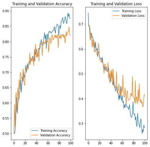
Now let’s plot the perfomance of the model on the two data sets.
acc = history.history['accuracy']
val_acc = history.history['val_accuracy']

loss = history.history['loss']
val_loss = history.history['val_loss']

epochs_range = range(EPOCHS)

plt.figure(figsize=(8, 8))
plt.subplot(1, 2, 1)
plt.plot(epochs_range, acc, label='Training Accuracy')
plt.plot(epochs_range, val_acc, label='Validation Accuracy')
plt.legend(loc='lower right')
plt.title('Training and Validation Accuracy')

plt.subplot(1, 2, 2)
plt.plot(epochs_range, loss, label='Training Loss')
plt.plot(epochs_range, val_loss, label='Validation Loss')
plt.legend(loc='upper right')
plt.title('Training and Validation Loss')
plt.savefig('./foo.png')
plt.show()
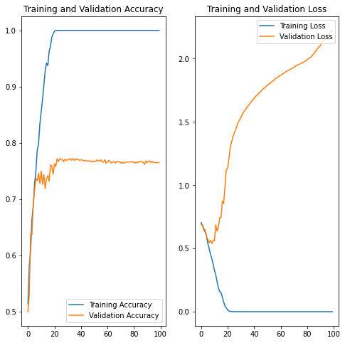
We see that after ca. 10 epochs the perfomance, of the model on the training and testing set, starts to diverge. This is a clear indication of overfitting. What we could do is to stop the training after ca. 10 epochs(early stopping). But let’s explore some alternatives to that.
Data Augmentation
When our dataset is limited we often run into the problem of overfitting. But what if we don’t have any more data, how can we handle that? One way is to augment the dataset we already have. We can apply random transformations to the images for instance: zoom, rotate and flip them horizontally.
We can apply these transformations using the ImageDataGenerator class.
Transformations
let’s see how the some of the transformations look like:
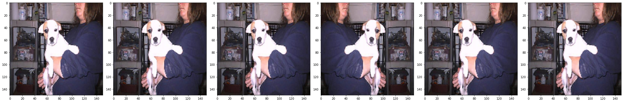
Horizontal flip
Here we take one figure and the transformation is applied randomly (or not).
image_gen = ImageDataGenerator(rescale=1./255, horizontal_flip=True)

train_data_gen = image_gen.flow_from_directory(batch_size=BATCH_SIZE,
                                               directory=train_dir,
                                               shuffle=True,
                                               target_size=(IMG_SHAPE,IMG_SHAPE))
augmented_images = [train_data_gen[0][0][0] for i in range(6)]
plotImages(augmented_images, 6)
Found 2000 images belonging to 2 classes.
Rotating
Here we demonstrate how rotate the image up to 45 degrees
image_gen = ImageDataGenerator(rescale=1./255, rotation_range=45)

train_data_gen = image_gen.flow_from_directory(batch_size=BATCH_SIZE,
                                               directory=train_dir,
                                               shuffle=True,
                                               target_size=(IMG_SHAPE, IMG_SHAPE))
Found 2000 images belonging to 2 classes.
augmented_images = [train_data_gen[0][0][0] for i in range(6)]
plotImages(augmented_images, 6)
Shear mapping
We can also apply a shear mapping to the figures
image_gen = ImageDataGenerator(rescale=1./255, shear_range=10)

train_data_gen = image_gen.flow_from_directory(batch_size=BATCH_SIZE,
                                               directory=train_dir,
                                               shuffle=True,
                                               target_size=(IMG_SHAPE, IMG_SHAPE))
augmented_images = [train_data_gen[0][0][0] for i in range(6)]
plotImages(augmented_images, 6)
Found 2000 images belonging to 2 classes.
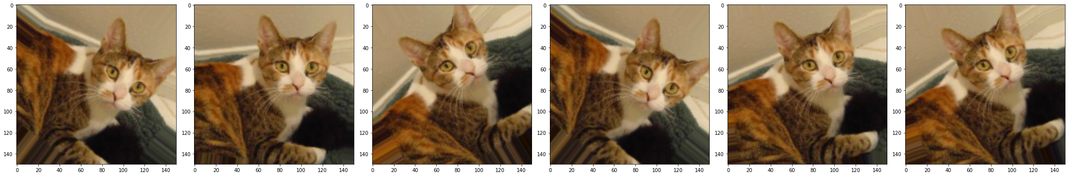
Final augmented dataset
Now we can apply all these transformations with one generator,so then this generator gives us batches from the “augmented” dataset.
image_gen_train = ImageDataGenerator(
      rescale=1./255,
      rotation_range=40,
      width_shift_range=0.2,
      height_shift_range=0.2,
      shear_range=0.2,
      zoom_range=0.2,
      horizontal_flip=True,
      fill_mode='nearest')

train_data_gen = image_gen_train.flow_from_directory(batch_size=BATCH_SIZE,
                                                     directory=train_dir,
                                                     shuffle=True,
                                                     target_size=(IMG_SHAPE,IMG_SHAPE),
                                                     class_mode='binary')
Found 2000 images belonging to 2 classes.
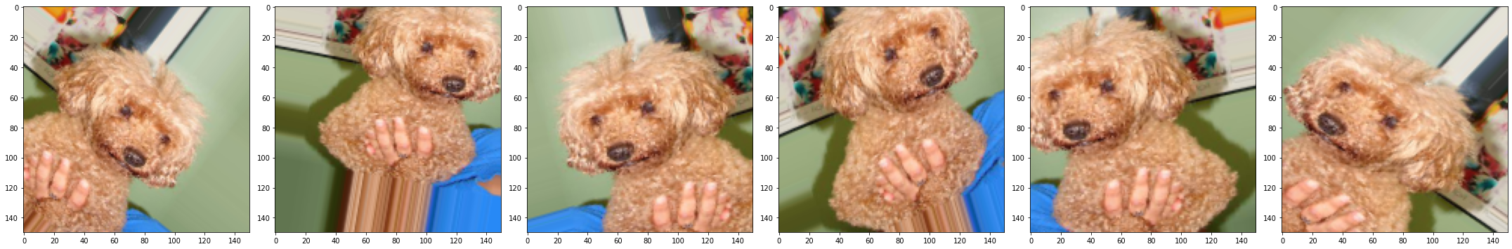
Let’s see a few examples
augmented_images = [train_data_gen[0][0][0] for i in range(6)]
plotImages(augmented_images, 6)
The generator for the validation dataset does not apply any transformations besides simply rescaling them and splitting into batches.
image_gen_val = ImageDataGenerator(rescale=1./255)

val_data_gen = image_gen_val.flow_from_directory(batch_size=BATCH_SIZE,
                                                 directory=validation_dir,
                                                 target_size=(IMG_SHAPE, IMG_SHAPE),
                                                 class_mode='binary')
Found 1000 images belonging to 2 classes.
Improving the model - Dropout
Now we have augmented the training dataset to help reduce overfitting. We can also improve the model itself to fight overfitting by applying dropout with probability of 50 %. Which means that 50% (randomly chosen) of the values coming into the dropout layers will be set to zero.
model = tf.keras.models.Sequential([
    tf.keras.layers.Conv2D(32, (3,3), activation='relu', input_shape=(150, 150, 3)),
    tf.keras.layers.MaxPooling2D(2, 2),

    tf.keras.layers.Conv2D(64, (3,3), activation='relu'),
    tf.keras.layers.MaxPooling2D(2,2),

    tf.keras.layers.Conv2D(128, (3,3), activation='relu'),
    tf.keras.layers.MaxPooling2D(2,2),

    tf.keras.layers.Conv2D(128, (3,3), activation='relu'),
    tf.keras.layers.MaxPooling2D(2,2),

    tf.keras.layers.Dropout(0.5),
    tf.keras.layers.Flatten(),
    tf.keras.layers.Dense(512, activation='relu'),
    tf.keras.layers.Dense(2)
])
model.compile(optimizer='adam',
              loss=tf.keras.losses.SparseCategoricalCrossentropy(from_logits=True),
              metrics=['accuracy'])
Now let’s just train the model
epochs=100
history = model.fit_generator(
    train_data_gen,
    steps_per_epoch=int(np.ceil(total_train / float(BATCH_SIZE))),
    epochs=epochs,
    validation_data=val_data_gen,
    validation_steps=int(np.ceil(total_val / float(BATCH_SIZE)))
)
Results of improved model
Now that we have used the augmented training dataset to train the improved (dropout) model Let’s look at its performance
acc = history.history['accuracy']
val_acc = history.history['val_accuracy']

loss = history.history['loss']
val_loss = history.history['val_loss']

epochs_range = range(epochs)

plt.figure(figsize=(8, 8))
plt.subplot(1, 2, 1)
plt.plot(epochs_range, acc, label='Training Accuracy')
plt.plot(epochs_range, val_acc, label='Validation Accuracy')
plt.legend(loc='lower right')
plt.title('Training and Validation Accuracy')

plt.subplot(1, 2, 2)
plt.plot(epochs_range, loss, label='Training Loss')
plt.plot(epochs_range, val_loss, label='Validation Loss')
plt.legend(loc='upper right')
plt.title('Training and Validation Loss')
plt.show()
We see that the accuracy goes up “almost” monotonically for both the training and validation set and the performance on the validation set is considerably better than before - simply by augmenting the dataset with simple transformations and adding dropout to the neural network.